This simple example shows how to calculate the input impedance of a simple cone.
The NumPy package is used for the array type while pylab for plotting.
>>> import numpy
>>> import pylab
We import the wiat package and the symbols from the subpackage TM. This is useful to avoid writing wiat.TM.xxx all the time
>>> import wiat
>>> from wiat.TM import *
An array of frequencies for which we want to calculate the impedance is created. It is important that the frequency vector be relatively fine for the various algorithm to works. Frequencies every 10 Hz works fine but we choose every 1 Hz here for nicer graphics.
>>> f = numpy.arange(50.,2000.,1.)
The temperature of the air inside the instrument. This value influence slightly the playing frequencies
>>> T = 25.
The definition of the instrument.
>>> a_cone = Instrument("A simple cone", [Cone(0.012,0.07,0.9)],
...                     UnflangedOpenEnd(0.07))
Calculate the impedance of the instrument for each frequencies.
>>> Z = CalculateImpedance(a_cone,f,T)
Find the exact locations of the first 3 maxima. This function uses an optimization algorithm and the results do not depend on the frequency vector, as far as it was fine enough to adequately represent the impedance function.
>>> maxima = CalculateMaxima(Z, a_cone, f, T, number_of_maxima=3)
>>> print 'Maxima no. - Frequency - Magnitude'
Maxima no. - Frequency - Magnitude
>>> for i,m in enumerate(maxima):
... print ' %d - %7.2f - %5.2f'%(i,m[0],m[1])
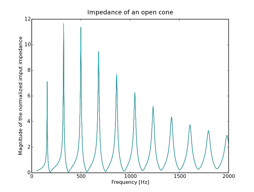
0 - 156.79 - 7.13
1 - 323.66 - 11.71
2 - 498.99 - 11.33
We can now plot of the impedance and save it to a file. We use a dummy variable to avoid seing the return value.
>>> dummy = pylab.plot(f,numpy.abs(Z))
>>> dummy = pylab.xlabel('Frequency [Hz]')
>>> dummy = pylab.ylabel('Magnitude of the normalized imput impedance')
>>> dummy = pylab.title('Impedance of an open cone')
>>> pylab.savefig('example1')
>>> # pylab.show()
You should now have a file called example1.png in the same directory.