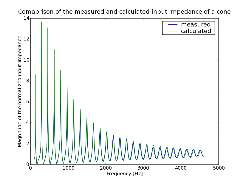
In this example, we compare the measured impedance of a cone with calculations.
We load the necessary modules.
>>> import os
>>> import numpy
>>> import pylab
And the wiat package
>>> import wiat
>>> from wiat.TM import *
Load the measured input impedance from a Matlab file. The measurement has been done with a two-microphone transfer function probe.
>>> f_meas,Z_meas = wiat.Data.load_from_mat(('freqs','z'),
...     wiat.MEASUREMENTDIR + os.sep + '2008-04-19Zshaped_open_cone.mat')
Calculate the approximate location of the maxima by interpolation in the data
>>> maxima_meas = wiat.Data.interpolate_maxima(f_meas,Z_meas)
Create the frequency array for the calculations.
>>> f = numpy.arange(100,4600,1,dtype=float)
>>> T = 25.
We can use a dictionary to store the parameters of the cone and pass it to the function
>>> ConeParameters = {'d0': 0.0125,'de': 0.0631,'L': 0.9652}
Define the instrument
>>> I = Instrument("Open cone", [Cone(**ConeParameters)],
...         UnflangedOpenEnd(ConeParameters['de']))
Calculate its input impedance
>>> Z_cone = CalculateImpedance(I,f,T)
Find the exact location of the first 5 maxima
>>> maxima_cone = CalculateMaxima(Z_cone,I,f,T,number_of_maxima=5)
Compare the measured and calculated maxima.
>>> maxima_comparison = CompareMaxima(maxima_meas, maxima_cone)
>>> print 'f1 [Hz] | f2 [Hz] | Interval [cents] | |Z1| | |Z2| | Ratio [dB]'
f1 [Hz] | f2 [Hz] | Interval [cents] | |Z1| | |Z2| | Ratio [dB]
>>> print '========|=========|==================|======|======|==========='
========|=========|==================|======|======|===========
>>> for c in maxima_comparison:
...     print '%7.2f | %7.2f | %+4.2f            | %4.1f | %4.1f | %+3.1f'%\
...           c[0:6]
 143.18 |  142.91 | -3.30            |  7.4 |  8.6 | +1.3
 297.82 |  298.27 | +2.60            |  8.5 | 13.7 | +4.1
 462.57 |  462.83 | +0.99            |  7.8 | 13.1 | +4.5
 631.48 |  632.17 | +1.88            |  7.1 | 11.0 | +3.8
 803.48 |  803.99 | +1.10            |  6.5 |  9.0 | +2.9
Plot the results
>>> dummy = pylab.plot(f_meas,numpy.abs(Z_meas),f,numpy.abs(Z_cone))
>>> dummy = pylab.legend(('measured','calculated'))
>>> dummy = pylab.xlabel('Frequency [Hz]')
>>> dummy = pylab.ylabel('Magnitude of the normalized input impedance')
>>> dummy = pylab.title(
...     'Comparison of the measured and calculated input impedance of a cone')
>>> pylab.savefig('example2')
>>> # pylab.show()
You should now have a file called example2.png in the same directory.