Bleed Through Removal Software
Authour: Cory McKay
Project Head: Ichiro Fujinaga
Last Update: September 10, 2004.
Overview
The goal of this project was to remove bleed through from pairs of greyscale scans of microfilms of Medieval and Renaissance scores. Some of the images of scores that are photographed from opposite sides (recto and verso) of the same physical piece of parchment or paper contain portions of the score on the opposite side of the paper or parchment which has bled through the paper. This bleed through complicates automated reading and parsing of the scores. In some cases, it makes even manual reading of portions of the score difficult or impossible. A further difficulty is that many of the microfilm images are high contrast, which complicates the task of recognizing the difference between bleed through symbols and normal symbols based only on shading.
The software developed for this project was designed in order to remove bleed through from the scores without corrupting the actual score into illegibility. This initial attempt makes use of global and localized thresholding algorithms to convert the greyscale images into binary images consisting only of white and black pixels where, hopefully, the bleed through areas have been converted to white along with the background and the actual symbols on the score have been converted to black. Although some encouraging success has been achieved, further research into additional methods is needed to further improve performance.
A prototype with a full GUI was implemented in Java. The techniques developed here are intended to eventually be integrated into the Gamera software framework.
Functionality
The functionality of this software was added to the ScoreReader software that had previously been developed for staff line detection. The original functionality of this software is still available in this version of ScoreReader, and is described here. The software is now able to perform the following additional tasks:
Screen Shots
|
|
|
|
Algorithm
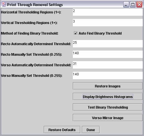
The following algorithm was used to convert a region (or all) of an image to a binary region:
The user has the option to divide the images into separate regions where different thresholds will be independently automatically determined, or may use a single automatically determined threshold for the entire image. The user may also manually specify a threshold.
Results
The following examples demonstrate the strengths and weaknesses of several variations of the thresholding described above:
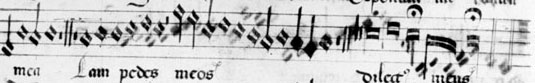 |
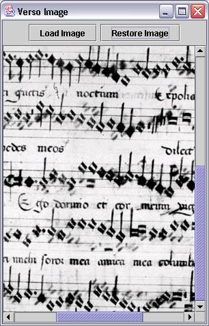
| Example 1a: Excerpt from the original image of a score scanned from microfilm. |
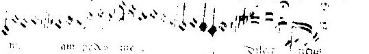 |
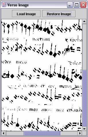
| Example 1b: Example 1a after conversion to a binary image using a single automatically determined threshold for image of the entire score. |
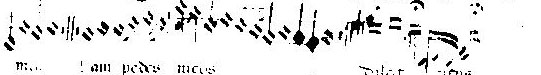 |
| Example 1c: Example 1a after conversion to a binary image using different automatically determined thresholds for different regions of the score. |
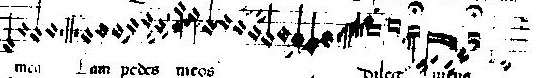 |
| Example 1d: Example 1a after conversion to a binary image using the default manually set threshold. |
Example 1a above shows a good deal of bleed through from the opposite side of the page. In this particular case, it is relatively easy for a human to determine what parts of the image are due to bleed through and which are not, but this task is not necessarily as easy for a computer. The use of a single automatically determined threshold, as shown in Example 1b, was effective in eliminating almost all of the bleed through, but also eliminated some potentially useful information, such as the score lines. The use of automatically determined regional thresholds managed to preserve more of the useful information than the global threshold did, as can be seen in a comparison of Examples 1b and 1c, but score lines were still lost for the most part, and a small amount of bleed through did manage to make it through the thresholding. The use of the default threshold, as shown in Example 1d, preserved almost all of the useful information, but also allowed a fair amount of bleed through to survive.
The loss of score lines is not in itself a critical problem, as these can likely be detected in the original image using a separate algorithm, and then added to the binary image after thresholding. This seems to indicate that automatic thresholding did a relatively good job. Whether a global threshold or regional thresholds are preferable depends on the robustness of the note recognition algorithm. Manual thresholding using the default value, which was arrived at through experimentation with a number of different scores, seems to be the poorest performer, as it lets through too much bleed through.
As one would expect, this thresholding approach was less effective in dealing with types of bleed through that were very dark, as can be seen below:
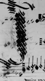 |
| Example 2a: Excerpt from original score. |
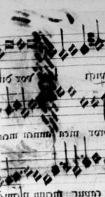 |
| Example 2b: Mirror image of corresponding section of original score on opposite side of page of score shown in Example 2a. |
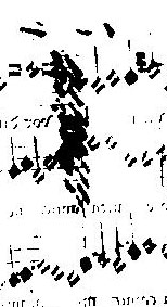 |
| Example 2c: Example 2b after conversion to a binary image using different automatically determined thresholds for different regions of score. |
The bleed through of the drop cap from Example 2a still has a significant portion remaining after thresholding, as can seen in Example 2c. Examples such as this, where the bleed through is as dark or darker than the correct note heads, cannot be solved by simple thresholding alone.
Possible Improvements
As can be seen in the results section, some encouraging results have been achieved with thresholding, but further research is needed to refine the results in order to arrive at a truly effective system. Some ideas for future are as follows:
Final processing could also be performed on the original image, with the knowledge gained from the binary image, where surviving pixels in the binary image are restored to their original colours and other pixels are set to the background colour.
Downloads
The software is available in a self-contained runnable Jar file here.
The source code and JavaDocs are available in a zipped file here.