Synthesizing piano Sustain Pedal Effect

Hanwen Zhang

2024 Fall MUMT618 Final Project

Abstract

This project explores the synthesis of piano sustain pedal effect, focusing on isolating and recreating such effect by modeling frequency-dependent decay behavior. We tried various approaches to synthesizing pedaled notes from unpedaled recordings.

Motivation

The piano sustain pedal affects the instrument's sound by holding the dampers above the strings, preventing them from cutting off vibrations. This allows the strings to vibrate freely after the keys are released. The sustain pedal is widely regarded as one of the most important aspects of piano playing, as it not only prolongs the notes but also introduces a variety of nuanced colors to the sound.

This project seeks to:

• Isolate and analyze the acoustical differences between pedaled and unpedaled piano sounds

• Develop methods for synthesizing realistic sustain pedal effect

• Find a way to efficiently make paired datasets suitable to train machine learning models for further research projects

(Diagram made with Microsoft PowerPoint)

Background and Related Work

Several research approaches have contributed to our understanding of piano sustain pedal effect:

Acoustical analysis

1. Heidi-Maria Lehtonen's work at Helsinki University of Technology (2007, 2009)

Physical modeling

2. Juliette Chabassier's comprehensive physical modeling of piano mechanics at École Polytechnique (2012, 2013)

Deep learning related approaches

3. DDSP-based modeling of expressive piano performance audio by Renault, Mignot, and Roebel at IRCAM (2022)

4. VirtuosoNet, an RNN-based System of modeling piano performance by Jeong et al. (2019)

5. Deep learning approach of synthesizing pedaling effect by Ching and Yang (2021)

Among the works listed above, [1] analyzes acoustic recordings of single notes played with and without the sustain pedal, including the case of partial pedaling (Lehtonen 2009). Lehtonen (2007) also proposes a synthesis algorithm for full pedal effect with parameters derived from the analysis of recordings. This algorithm incorporates 12 string models and resembles the structure of a reverberation algorithm, a common practice for piano synthesis, as noted by the author. In contrast, [2] adopts a comprehensive physical modeling approach for the whole grand piano, including potentially all components such as the soundboard, string-hammer interactions, and pedals. The result is a complicated system with many partial differential equations. Notably, the author, Juliette Chabassier, later worked for Modartt, the company behind Pianoteq.

Although recent approaches start to adopt deep learning techniques, largely enabled by the E-Piano Competition dataset, which provides paired audio recordings and synchronized MIDI data for approximately 200 hours (Hawthorne, 2019), the results remain far from ideal. The synthesized sound quality is still not comparable to real recordings. For instance, [3] aims to recreate expressive performance details from MIDI input, but their output audio samples lack the natural quality of original recordings. While the audio samples linked in [4] are no longer accessible, their listening tests also highlight the discrepancy between the synthesized output and the expected real sound from a human pianist. Similarly, while [5] narrowed the synthesis task specifically to pedaling effects, the results suggest a lot of potential for improvement.

These efforts demonstrate several limitations in current deep learning approaches:

• There is insufficient training data for expressive piano performance with accurate annotations.

• At present, physical models and sample-based models still remain the most reliable options for producing high-quality, realistic piano sound synthesis.

Data Collection

To obtain paired recordings, we initially faced several challenges. Ideally, recordings would be made in an anechoic chamber to avoid unwanted reverb and noise. However, it is still difficult to achieve identical excerpts played by a human, so we opted to use MIDI information to control a Yamaha Disklavier while simultaneously recording the audio. A critical question arises: how many pairs of recordings do we need? Theoretically, it could follow the pattern 88 + 88*87 + …, considering all possible combinations. While the MAESTRO dataset (Hawthorne 2019) is a valuable resource, complete performance recordings are too complex for our purposes. To overcome these issues, we wrote MIDI scripts and passed them into Pianoteq, a complete physical model of the grand piano developed at the Institute of Mathematics of Toulouse. This approach offers several advantages:

• Option for no room reverb or background noise

• Precise control over note timing and velocity

• Perfect alignment between pedaled and unpedaled versions

• Consistent recording conditions using a simulated Steinway D piano

Recording parameters (MIDI script generated by make_midi.py):

• Velocity: 100 (consistent across all samples)

• Note press duration: 0.2 seconds (to simulate finger press)

• No reverb or other effects

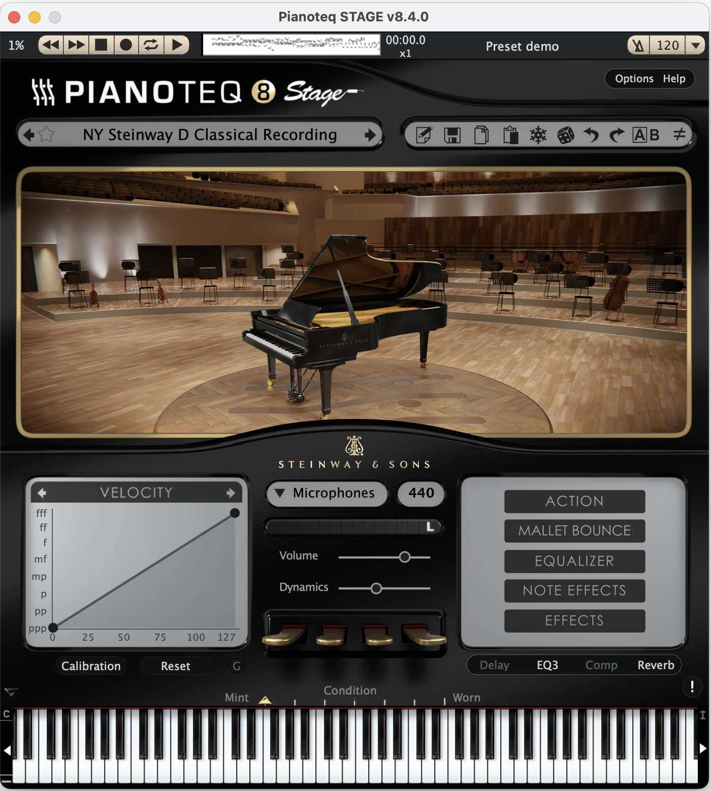
The interface of Pianoteq v8.4.0:

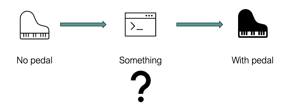
Here we need to compare the three types of single notes and we will come back to these three types later:

a. Play and release

b. Play and hold $\approx$$\approx$ Play and release but hold the damper for the played note with sostenuto pedal

c. Play and release but hold all dampers with sustain pedal

Question: Sustain pedal effect = sustain + sympathetic vibration ?

Synthesis Methods

Method 1: Lehtonen's Synthesis (2007)

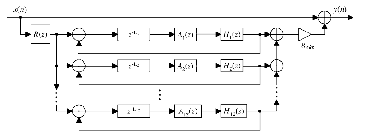
Here is the main structure of this systhesis algorithm:

• 12 simplified string models for the lowest piano strings, and the length of each delay line is determined by frequency

  $L_k=\text{floor}(\frac{f_s}{f_{0,k}}+\frac{1}{2})$$L_k=\text{floor}\left(\frac{f_s}{f_{0,k}}+\frac{1}{2}\right)$ where $f_s$$f_s$ is the sampling frequency, $f_{0,k}$$f_{0,k}$ is the fundamental frequency of the tone for string $k$$k$. The algorithm is developed using 12 lowest strings, which are supposed to have the most partials, to save the computational cost. In fact, when tested against a commercial practice of 18-string models, Lehtonen's system exhibits better performance in the listening test for low and high range of the piano but less in the middle range.

• Dispersion filter (A) to spread the harmonic components of the string models more randomly in the sympathetic spectrum. The transfer function is designed as $A_k(z)=\frac{a_{1,k}+z^{-1}}{1+a_{1,k}{z}^{-1}}$$A_k(z)=\frac{a_{1,k}+z^{-1}}{1+a_{1,k}z^{-1}}$ where $a_{1,k}=\frac{1-D_k}{D_k+1}$$a_{1,k}=\frac{1-D_k}{D_k+1}$ and $D_k$$D_k$ is the phase delay value at dc and approximated by $D_k=2\sqrt{B_k}$$D_k=2\sqrt{B_k}$ with measured inharmonicity parameter $B_k$$B_k$ for each string $k$$k$.

• A first-order lowpass filter (H) for frequency-dependent loss with transfer function $H_k(z)=\frac{b_k}{1+c{z}^{-1}}$$H_k(z)=\frac{b_k}{1+cz^{-1}}$ with $b_k=g_k(1+c)$$b_k=g_k(1+c)$ so that the overall decay and the frequency-dependent decay are controlled by $g_k$$g_k$ and $c$$c$, respectively.

• Tone correction filter (R) for residual energy modeling as $R(z)=\frac{0.1164(1-z^{-1})}{1-1.880z^{-1}+0.8836z^{-2}}$$R(z)=\frac{0.1164(1-z^{-1})}{1-1.880z^{-1}+0.8836z^{-2}}$.

We implemented this system in MATLAB in Lehtonen.m and added a normalization step at the end to prevent clipping.

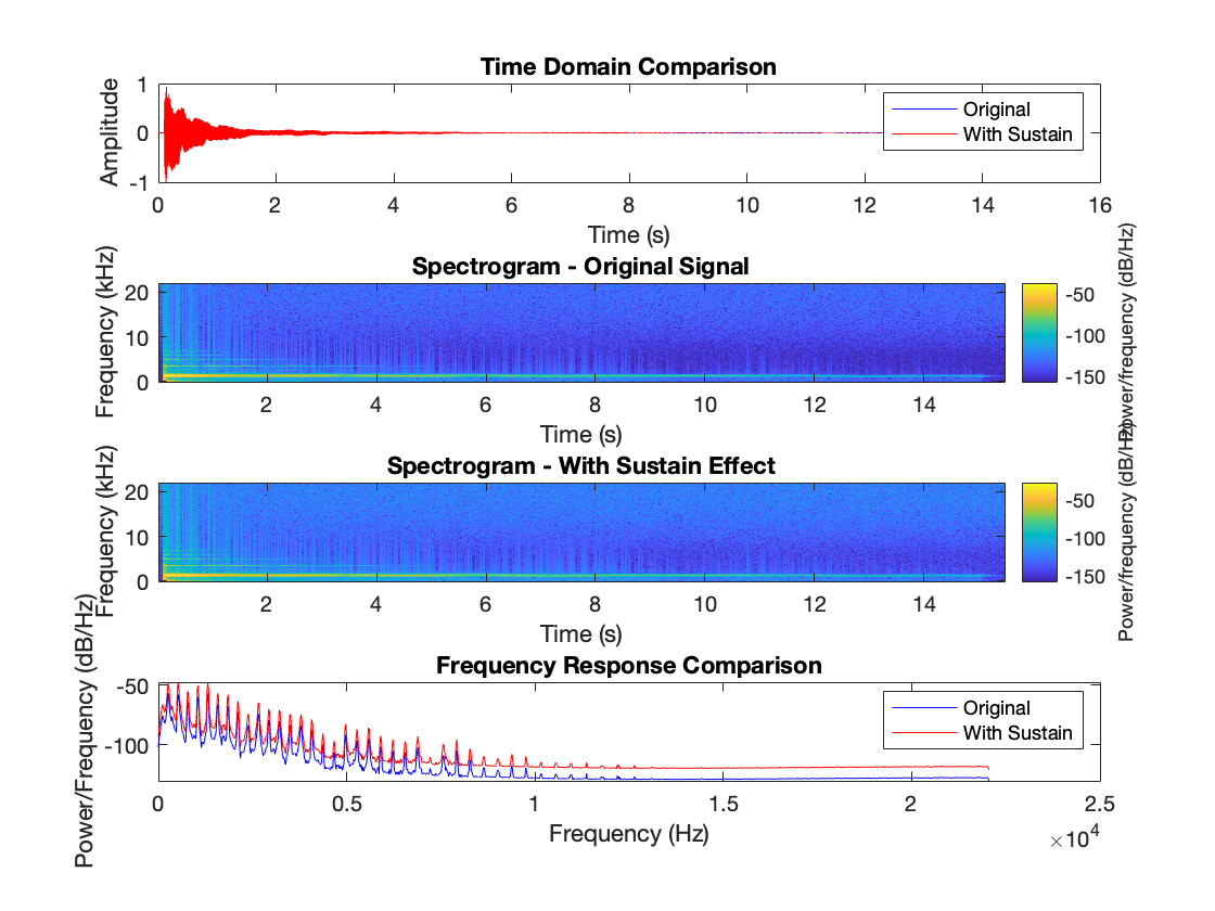
As shown in the plot below, for middle C (MIDI number 60), the implementation of the piano sustain pedal effect shows some success but also has limitations. In the time-domain plot (top), we can see that the synthetic sustain effect maintains a longer decay compared to the original signal, which is expected. However, the spectrograms (middle plots) reveal that the effect doesn't introduce much sympathetic vibration, as we would expect from a real piano sustain pedal. Ideally, there should be more energy visible between the harmonic partials. The frequency response comparison (bottom) shows increased energy levels across frequencies in the sustained version (red line), but the pattern appears somewhat artificial. The peaks are too regular, and the valleys between harmonics aren't filled in as they might be with the sympathetic vibration. A real piano sustain pedal would create more complex interactions between strings, resulting in a denser spectrum with more energy between the main harmonics. This suggests that while the basic sustain mechanism is functioning, the current implementation isn't fully capturing the intricate string coupling and resonance behaviors that make a real piano's sustain pedal so rich and musical. The effect seems to primarily extend decay times rather than create true sympathetic resonances. Additionally, our Pianoteq recording differs from the YAMAHA concert grand used in Lehtonen's experiment, meaning the parameters are not quite exact, not to mention the potential inaccuracy in the Pianoteq program as well.

However, more importantly, this method is only working for a single note and the input signal is already "sustained by finger" rather than a real play-and-release short note. Therefore, this algorithm realizes synthesis from [b] to [c] while we ultimately want to go from [a] to [c]. To our knowledge, this has not received much research attention.

Method 2: Deconvolution

Plan

1. Deconvolve the paired pedaled and non-pedaled recordings.

2. Analyze the impulse response generated by the deconvolution process.

3. Convert the resulting impulse response into a filter that can be applied to non-pedaled audio.

Problem(s): The deconvolution process does not work directly in the time domain, resulting in a very large residual and preventing the computation from terminating.

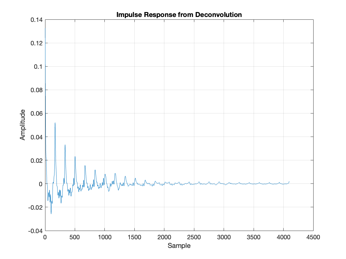
Attempt: To address the issue, the impulse response was reconstructed in the frequency domain, then transformed back into the time domain. The impulse response was then convolved with the non-pedaled audio and combined with the original audio to approximate the sound produced with the sustain pedal. The code provided implements this process using a MIDI script, where parameters such as window size, FFT size, and scaling factor are defined. The analysis begins by selecting analysis chunks in the loaded audio files (both pedaled and non-pedaled). The spectral differences between the pedaled and non-pedaled audio are calculated to create the frequency difference profile, which is then used to build the impulse response. The reconstructed impulse response is applied to the non-pedaled audio using convolution to approximate the pedaled sound. The code can be found in IR.m.

 

 

Analysis:

The fundamental issue with this approach is that we're trying to treat the piano's sustain pedal like a simple effect that can be captured through deconvolution. While we tried increasing the analysis window to 3000 samples, the core problem remains: the sustain pedal creates complex interactions between strings that cannot be modeled as a simple filter.

Looking at our results:

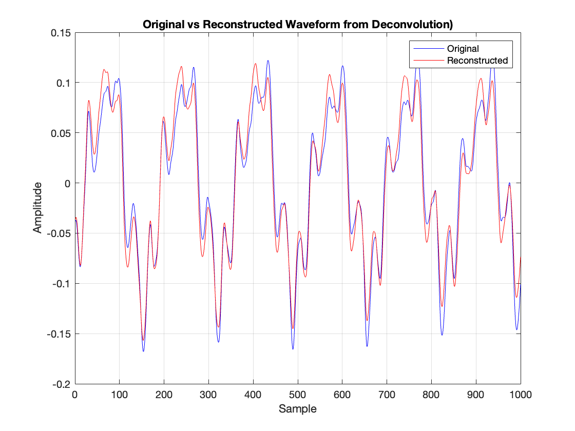
1. The reconstruction plot shows timing misalignments - the blue and red lines don't perfectly match because our frequency-domain subtraction ignores important phase information.

2. The amplitude differences between original (blue) and reconstructed (red) signals indicate that simply adding filtered sound to the original note isn't enough to recreate how strings actually interact when the pedal is pressed.

3. We're attempting to represent a complex, interactive system with a single, fixed filter - but the real pedal effect involves strings responding to each other in ways that change over time.

This is why we see the large residual error mentioned in the first attempt - the actual physics of sympathetic string resonance cannot be captured by this simplified linear model.

Method 3: Peak Detection and Decay Curve Fitting

Step 1: Analysis

1. The frequency spectrum is divided into 20 logarithmically spaced bands: $f_k=f_{min}\ast (f_{max}/f_{min}{)}^{k/N}$$f_k = f_{min} * (f_{max}/f_{min})^{k/N}$ where $f_{min}=50$$f_{min} = 50$ Hz, $f_{max}=f_s/2$$f_{max} = f_s/2$ and $N=20$$N = 20$ bands.

2. (Peak Detection) For each frequency band, up to 15 peaks are detected using magnitude spectrum analysis $P(\omega )=|S(t,\omega )|$$P(ω) = |S(t,ω)|$ (magnitude spectrum from the Short-Time Fourier Transform).

3. (Decay Rate Estimation) For each detected mode:

   • Extract the magnitude envelope: $E(t)=|S(t,{\omega }_i)|$$E(t) = |S(t,ω_i)|$

   • Convert to logarithmic scale: $E_{log}(t)=\ln (E(t)+\epsilon )$$E_{log}(t) = \ln(E(t) + ε)$

   • Fit linear decay: $E_{log}(t)\approx \alpha t+\beta$$E_{log}(t) ≈ αt + β$

   • Decay rate: $r_i=max(-\alpha ,0.05)$$r_i = \max(-α, 0.05)$

4. Frequency-Dependent Modifications

   • Decay rates are modified based on frequency: $r_i^{\prime }=r_i(0.5+0.5e^{-f_i/1000})$$r_i' = r_i(0.5 + 0.5e^{-f_i/1000})$

   • Amplitudes are weighted: $A_i^{\prime }=A_i{e}^{-f_i/2000}$$A_i' = A_i e^{-f_i/2000}$

Step 2: Synthesis

1. The synthesized signal combines:

   • Attack portion from input recording (type [a], play-and-release) with smooth transition.

   • Synthesized decay $y(t)=\sum _{i=1}^N{A}_i{e}^{-r_i^{\prime }t}\cos (2\pi f_{i}t+{\phi }_i+\eta (t))$$y(t) = \sum_{i=1}^{N} A_i e^{-r_i't} \cos(2πf_it + φ_i + η(t))$ where: $A_i$$A_i$ is the mode amplitude, $r_i^{\prime }$$r_i'$ is the modified decay rate, $f_i$$f_i$ is the mode frequency, ${\phi }_i$$φ_i$ is the initial phase and $\eta (t)$$η(t)$ is small random perturbation ($\sim \mathcal{N}(0,0.0001)$$\sim \mathcal{N}(0, 0.0001)$).

2. (String Coupling) For modes within 50 Hz, $y_i(t)=y_i(t)+\sum _{j\ne i}{c}_{ij}{A}_j{e}^{-r_j^{\prime }t}\cos (2\pi f_{j}t+{\phi }_j)$$y_i(t) = y_i(t) + \sum_{j≠i} c_{ij}A_j e^{-r_j't} \cos(2πf_jt + φ_j)$, where coupling coefficient $c_{ij}=0.2e^{-|f_i-f_j|/10}$$c_{ij} = 0.2e^{-|f_i-f_j|/10}$.

3. (Envelope Matching) 20 logarithmically spaced bands using Butterworth filters:

   • Lowpass: $H_1(s)=\frac{{\omega }_c^2}{s^2+\sqrt{2}{\omega }_{c}s+{\omega }_c^2}$$H_1(s) = \frac{ω_c^2}{s^2 + \sqrt{2}ω_cs + ω_c^2}$

   • Bandpass: $H_k(s)=\frac{\sqrt{{\omega }_2-{\omega }_1}s}{s^2+({\omega }_2-{\omega }_1)s+{\omega }_2{\omega }_1}$$H_k(s) = \frac{\sqrt{ω_2-ω_1}s}{s^2 + (ω_2-ω_1)s + ω_2ω_1}$

   • Highpass: $H_N(s)=\frac{s^2}{s^2+\sqrt{2}{\omega }_{c}s+{\omega }_c^2}$$H_N(s) = \frac{s^2}{s^2 + \sqrt{2}ω_cs + ω_c^2}$

   For each band:

   • Calculate RMS envelope (using a window of 0.1 seconds): $E_{RMS}(t)=\sqrt{\frac{1}{W}\sum _{n=0}^{W-1}{x}^2(t+n)}$$E_{RMS}(t) = \sqrt{\frac{1}{W}\sum_{n=0}^{W-1} x^2(t+n)}$

   • Compute scaling factor: $S(t)=\frac{E_{target}(t)}{E_{synth}(t)+\epsilon }$$S(t) = \frac{E_{target}(t)}{E_{synth}(t) + ε}$

   • Apply smoothed scaling: $y^{\prime }(t)=y(t)+(y_{\text{band}}(t)S_{\text{smoothed}}(t)-y_{\text{band}}(t))$$y'(t) = y(t) + \left(y_{\text{band}}(t)S_{\text{smoothed}}(t) - y_{\text{band}}(t)\right)$ , where $S_{smoothed}$$S_{smoothed}$ is filtered with a Gaussian window

There was no particular reason or existing architecture to follow. Mostly trial and error trying to fit the spectrogram. The code is method3.m.

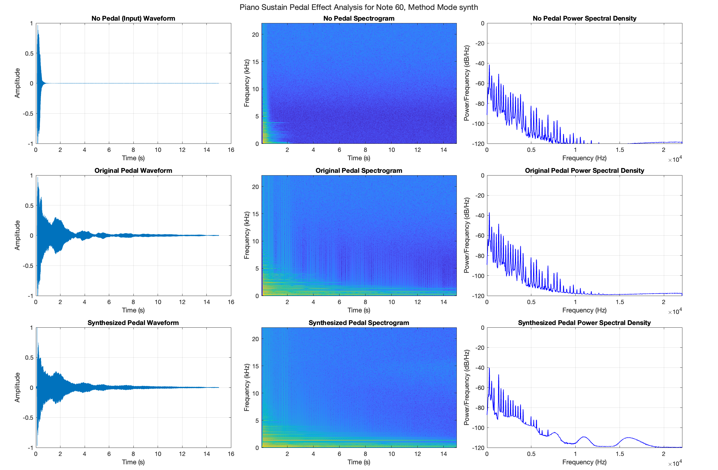
Looking at the three rows of plots comparing the no-pedal, original pedal, and synthesized pedal signals, the temporal waveforms (left column) indicate the fundamental difference between non-pedaled and pedaled recordings, where the sustain pedal extends the decay envelope significantly. The synthesized version's waveform closely matches the original pedaled version's overall envelope shape due to the multi-band envelope matching process implemented in the synthesis step. The spectrograms (middle column) plot the frequency content over time: without pedal, we see rapid decay across all frequencies; with pedal, there's extended resonance and complex harmonic interactions. The synthesized version attempts to replicate this pedaled behavior but shows some artificial characteristics, particularly in its more uniform decay pattern. The power spectral density plots (right column) highlight limitations in the synthesis, especially above 15 kHz where irregular peaks appear, which are not present in the original pedaled recording. These differences suggest that while the synthesis step captures the basic temporal extension of the sustain pedal through envelope matching, it does not fully reproduce the natural resonance characteristics and complex frequency interactions of a real piano.

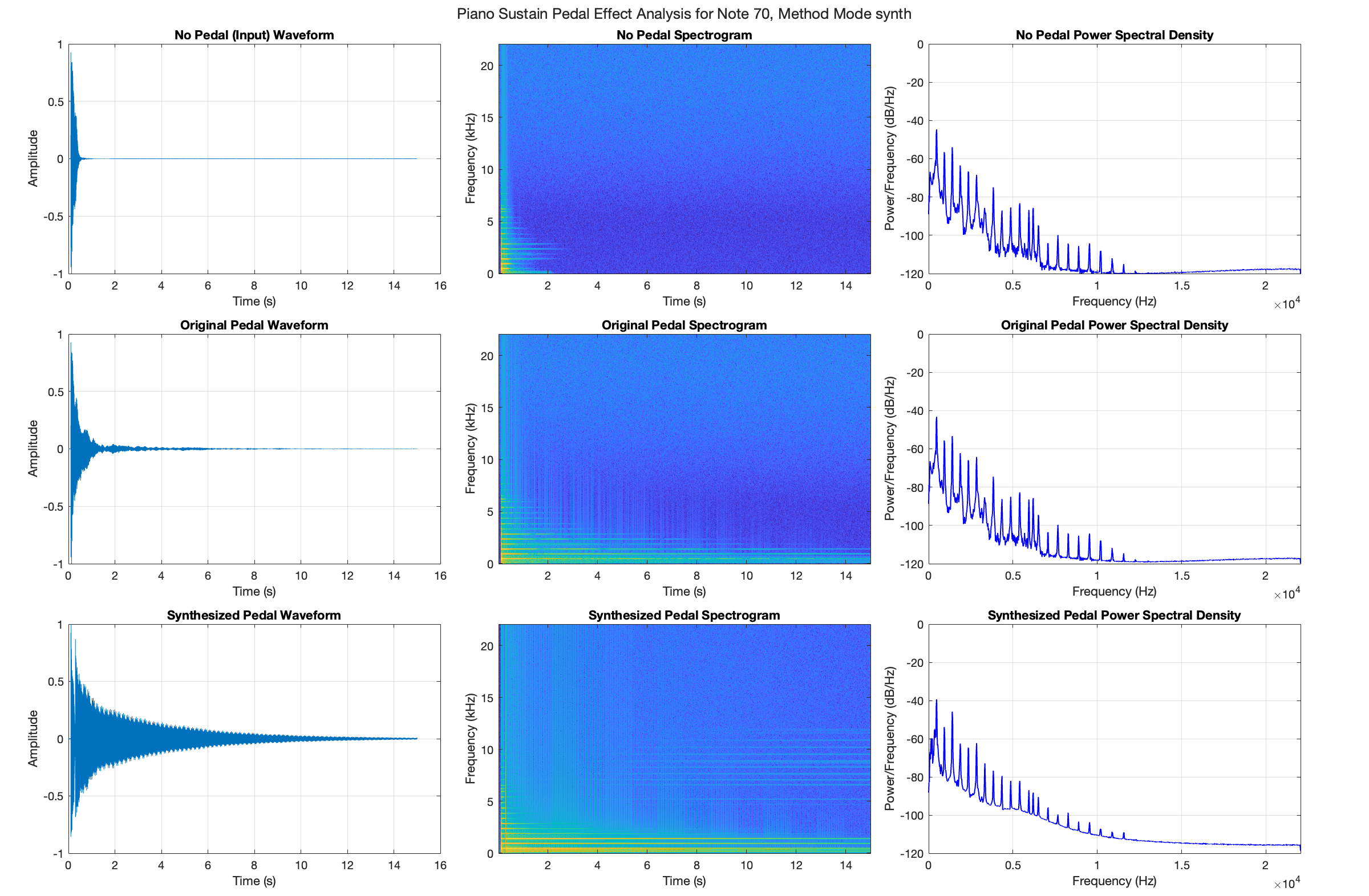
The synthesis performance also varies significantly across different piano notes, even for the note within the same octave (see the figure below for MIDI 70). Theoretically, low notes have longer, thicker strings with more complex vibrational modes, while high notes have shorter, thinner strings with simpler vibration patterns. This implementation works best for middle C, but a key limitation is the use of fixed parameters that do not adapt to different frequency ranges: the 20 frequency bands, 15 modes per band, 50 Hz coupling distance, and fixed decay rate modifications do not scale appropriately across the piano range. For instance, a 50 Hz coupling distance that works well for middle C would be too wide for higher notes and too narrow for lower notes, since harmonic spacing changes with the fundamental frequency. Resolution issues also arise where the frequency bands might be too wide to capture closely spaced harmonics in low notes, while the fixed number of modes might be insufficient for high notes' rapid decay. The envelope matching process, using a fixed window length (0.1 * fs), presents another limitation - potentially too long for fast-decaying high notes yet too short to capture the slow evolution of low notes. These issues suggest the need for adaptive parameters based on note frequency, variable frequency band division, and flexible envelope matching strategies to achieve consistent performance across the full range of piano. Furthermore, when the signal gets very quiet toward the end, dividing by small values (synth_env + eps) in envelope scaling could amplify noise, as we see in the spectrogram in the bottom.

Demo

Method	Input	Output (Synthesized)
1 (Lehtonen)	Play and hold	Play and pedal
3 (Fit decay curves)	Play and release	Play and release with pedal

Real pedaled recording (target):

Future Work

The next step would be to study different ways pianists use the pedal. This study only looked at basic pedal use, but real piano playing involves more complex techniques. For example, pianists might press the pedal before, during, or after hitting the keys. We're especially interested in part pedaling - where the pedal is pressed halfway down. This creates subtle sound changes that are important for expressive playing but hard to recreate digitally. Despite the recent interest in deep learning, Lehtonen's work based on acoustical analysis (2009) is still a good place to start.

For better research, we can use a Yamaha Disklavier, passing MIDI data to make it play notes and move the pedal exactly how we want while making the audio recordings. This would help us test different pedal techniques while keeping everything else the same. We could then study how the pedal works with more than just single notes - like when playing chords or fast passages, which is more like real music.

Furthermore, we need to better understand two different things that happen when using the pedal: strings vibrating in response to other strings (sympathetic vibration), and the way sound bounces around the room (reverbration). These work together to create the final sound. Also, pianists change how they use the pedal based on the room acoustics - they might use less pedal in a wet echoing concert hall. Future models should take this into account as well.

References

•Bank, Balazs, and Juliette Chabassier. 2019. “Model-Based Digital Pianos: From Physics to Sound Synthesis.” IEEE Signal Processing Magazine 36 (1): 11. https://doi.org/10.1109/MSP.2018.2872349.

•Chabassier, Juliette. 2012. “Modélisation et Simulation Numérique d’un Piano Par Modèles Physiques.” Theses, Ecole Polytechnique X. https://pastel.hal.science/pastel-00690351.

•Chabassier, Juliette, Antoine Chaigne, and Patrick Joly. 2013. “Modeling and Simulation of a Grand Piano.” The Journal of the Acoustical Society of America 134 (1): 648–65. https://doi.org/10.1121/1.4809649.

•Ching, Joann, and Yi-Hsuan Yang. 2021. “Learning to Generate Piano Music With Sustain Pedals.” In Extended Abstracts for the Late-Breaking Demo Session of the 22nd Int. Society for Music Information Retrieval Conf. (ISMIR). Online: International Society for Music Information Retrieval.

•Hawthorne, Curtis, Andriy Stasyuk, Adam Roberts, Ian Simon, Cheng-Zhi Anna Huang, Sander Dieleman, Erich Elsen, Jesse Engel, and Douglas Eck. 2019. “Enabling Factorized Piano Music Modeling and Generation with the MAESTRO Dataset.” In Proceedings of the 7th International Conference on Learning Representations. New Orleans, LA, USA: arXiv. http://arxiv.org/abs/1810.12247.

•Jeong, Dasaem, Taegyun Kwon, Yoojin Kim, and Juhan Nam. 2019a. “Graph Neural Network for Music Score Data and Modeling Expressive Piano Performance.” In Proceedings of the 36th International Conference on Machine Learning, edited by Kamalika Chaudhuri and Ruslan Salakhutdinov, 97:3060–70. Proceedings of Machine Learning Research. PMLR. https://proceedings.mlr.press/v97/jeong19a.html.

•———. 2019b. “VirtuosoNet: A Hierarchical RNN-Based System for Modeling Expressive Piano Performance.” In Proceedings of the 20th International Society for Music Information Retrieval Conference (ISMIR), 908–15. Delft, Netherlands: International Society for Music Information Retrieval Conference (ISMIR). http://hdl.handle.net/10203/269876.

•Lehtonen, Heidi-Maria, Anders Askenfelt, and Vesa Välimäki. 2009. “Analysis of the Part-Pedaling Effect in the Piano.” The Journal of the Acoustical Society of America 126 (2): EL49–54. https://doi.org/10.1121/1.3162438.

•Lehtonen, Heidi-Maria, Henri Penttinen, Jukka Rauhala, and Vesa Välimäki. 2007. “Analysis and Modeling of Piano Sustain-Pedal Effects.” The Journal of the Acoustical Society of America 122 (3): 1787–97. https://doi.org/10.1121/1.2756172.

•Modartt. 2024. “Pianoteq v8.4.0.” https://www.modartt.com/pianoteq.