Next: Audio Processing in Matlab Up: Signal Spectra Previous: The FFT
 FFT (or DFT) computes sinusoidal “weights” for evenly spaced frequencies between 0 and
 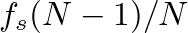 . From the sampling theorem, only the first half of these frequency weights are unique.
, the more sinusoidal weights are computed and the smaller the spacing between frequency components. This spacing is given by  .
.
) also represents the minimum non-zero frequency that can be resolved using a length DFT.
to get a more precise estimate of the frequency content.
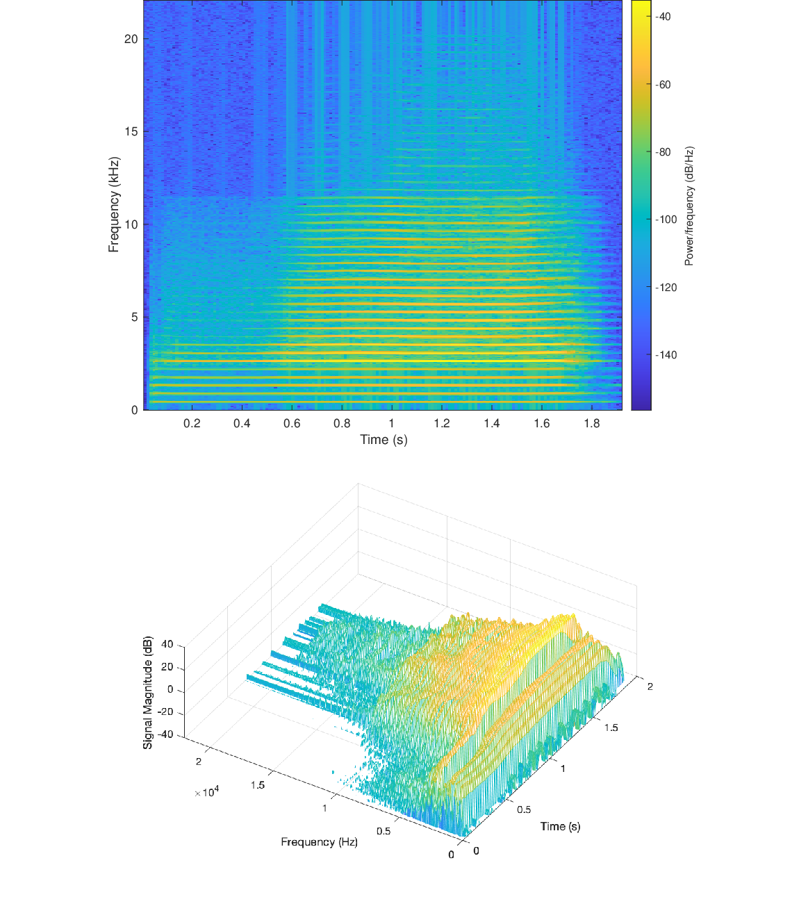
, in order to isolate changes over time.
 |

| ©2004-2024 McGill University. All Rights Reserved. Maintained by Gary P. Scavone. |