Next: ADSR Envelopes Up: Audio Envelopes and Decibels Previous: Linear Envelopes
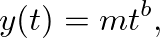
 is a scale factor calculated in a similar way to the linear line slope given above and
  is a curvature constant greater than zero.
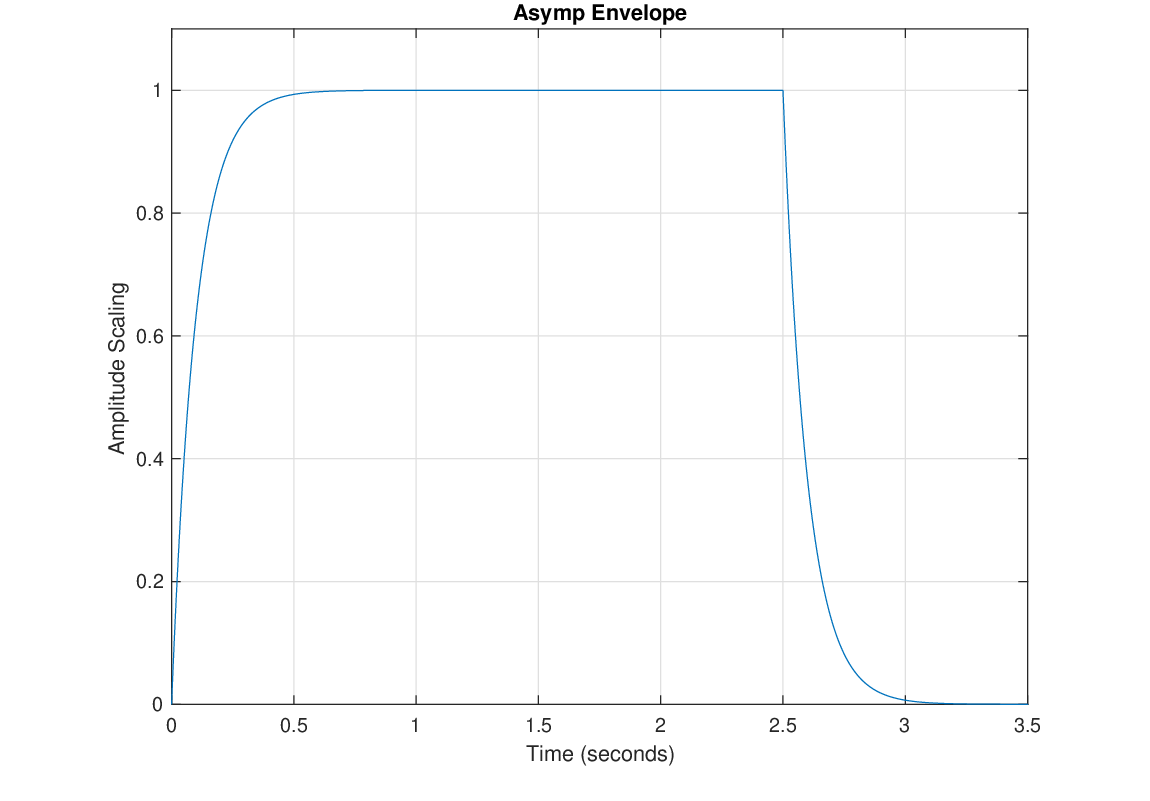
less than 1.0 produce "logarithmic" growth and exponential decay patterns. Values of greater than 1.0 produce exponential growth and "logarithmic" decay patterns. A value of  corresponds to linear growth and decay.
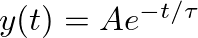 , remembering that exponential curves increase/decrease in equal proportion to their current value. This suggests an algorithm of the form:
![$\displaystyle y[n] = a y[n-1] + (1-a) \mbox{target},
$](img55.png)
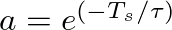 ,
,  is the sample period, and
  is a user provided time constant.

| ©2004-2024 McGill University. All Rights Reserved. Maintained by Gary P. Scavone. |