MUMT 618: Reading and Assignments
"Collaboration" Policy: Students can often learn a great deal from their peers. Feel free to seek help from other students (as well as the instructor) when you are having difficulty. But DO NOT COPY assignments. I expect you to write your own derivations, scripts, and code.
Matlab and C++ Code Remarks: Your Matlab and C++ programs should be easy to read and understand. At the top of each program, provide the program name, your name, and information about the program and how to use it. For C++ programs, included a g++ compiler statement that can be used to compile the program in the working directory. In your code, be liberal with comments. Even when a program does not execute properly, partial credit may be given based on comments that show good understanding of the issues and ways to approach the solutions. Use the C++ style guide to uniformly format your code.
| Week 8: Homework #6 | Due via email by class time on Thursday, 14 November 2024 |
- In Matlab, use frequency-domain, transmission-matrix techniques to calculate and plot the input impedance of a sequence of 3 cylindrical sections with the following dimensions: radii = 0.015, 0.01, and 0.008 meters, lengths = 0.02, 0.07, 0.09 meters. The Matlab script ZinMatrix.m should help you get started. You will also need the script reflpoly.m. [10 pts]
- In Matlab, implement a digital waveguide model of the three-segment cylindrical pipe structure defined above and calculate both the impulse response and input impedance of the structure. Ignore viscothermal losses. The Matlab script ZinWaveguide.m should help you get started. [10 pts]
- Course Text: pages 359-376, 383-400.
| Week 6: Homework #5 | Due via email by class time on Thursday, 24 October 2024 |
- Homework #5 (PDF)
- Course Text: pages 251-277, 459-468.
| Week 5: Homework #4 | Due via email by class time on Thursday, 3 October 2024 |
- Write a Matlab script or an STK program that implements the Karplus-Strong algorithm, including the drum algorithm with blend factor. The fundamental frequency, time duration, and blend factor of the computation should be specified at the top of the script. It is not necessary to implement the stretch factor, however, the algorithm should be extended to allow a fractional delayline length using allpass interpolation. If using STK, you should only need to use the DelayA, Noise, and OneZero classes for the algorithm itself. The output can either be in realtime to the DAC or to a soundfile. [7 pts]
- Course Text / Reading: pages 533-560.
- Prepare a short class project proposal and also propose a research paper to present in class (to be emailed to instructor).
- Karplus, K. and Strong, A. "Digital Synthesis of Plucked String and Drum Timbres," Computer Music Journal, 7(2), 1983, pp. 43-55.
- Jaffe, D. A. and Smith, Julius O., "Extensions of the Karplus-Strong Plucked String Algorithm," Computer Music Journal, 7(2), 1983, pp. 56-69.
- Course Text / Reading: pages 203-223.
| Week 3: Homework #3 | Due via email by class time on Thursday, 19 September 2024 |
- Write a Matlab script or an STK program (using existing classes) to create one of the following effects: Flanger, Doppler Shift (must involve a varying source-listener velocity over time) or Pitch Shifter. The script or program should take a soundfile as input and write the effected sound to a new output soundfile. [7 pts]
- Write a Matlab script that implements a basic late field feedback delay network artificial reverberation algorithm (without early reflections). Use a Householder mixing matrix, as described in the course notes, and design the system with N = 8 feedback channels (you can increase that if you wish), each having a one-pole lowpass filter. Specify values of T60 at frequencies of 0 and fs/2 at the top of the script that are subsequently used when parameterizing the lowpass filters. The delayline lengths should be prime numbers in the range from 1000 - 5000 samples at a sample rate of 44100 samples per second. The script should either use a unit impulse as input to the reverberator or take a soundfile as input and write the reverberated response to a new output soundfile. To simplify the process, you can use the filter() function to implement the delay lines and lowpass filters (see the following example). [8 pts]
- Course Text / Reading: pages 85-119.
| Week 2: Homework #2 | Due via email by class time on Thursday, 12 September 2024 |
Show how you perform your calculations for all the following questions.
- Read J. A. Moorer "About this reverberation business," Computer Music Journal, Vol. 3, No. 2, pp. 13-18, 1979.
- Assuming sound propagates at c = 343 meters per second (at 20 degrees Celsius), find the delay-line length M that can be used to simulate sound propagation delay over a distance of approximately 10 meters (rounded to the nearest sample), where the simulation sampling rate is 44.1 kHz. [1 pt]
- Suppose that pressure-wave amplitude was observed to decay by a factor of 2 in the geometry of the previous problem. In other words, sound propagation over a distance of 10 meters is associated with 6.02 dB of loss at all frequencies. What is the loss, specified as both a linear gain factor and in dB, associated with propagation over one spatial sample? [1 pt]
- Sketch a delay-line simulation of an acoustic point-source at p1 = (1, 1, 0) meters, a listener at p2 = (2, 0, 0), a reflecting wall at w1 = (x, 2, z), and a second reflecting wall at w2 = (0, y, z). Assume the wall reflection coefficient is 1, and that air absorption is 0.1 dB per meter at all frequencies. Assume the wave propagation is spherical, with appropriate scaling factors. [5 pts]
- (a) Find all acoustic path lengths in meters.
- (b) Find all acoustic path gains as linear scale factors.
- (c) Assuming sound speed is c = 343 meters per second, and the sampling rate is 44.1 kHz, find all delay-line lengths in samples (rounded).
- (d) Find the transfer function from source to listener with the direct path normalized out of the result.
- (e) Provide Matlab code to plot the echogram (impulse response) and amplitude response (magnitude frequency response).
- Add interpolation (either linear or allpass) functionality to your Matlab delay-line implementation from Homework #1. The interpolation operation should happen inside your delay loop without making use of the filter function (i.e., implement your own filtering difference equation). Include a test of this functionality in the script. [5 pts]
| Week 1: Homework #1 | Due via email by class time on Thursday, 5 September 2024 |
- Course Text / Reading: pages 37-49, 57-63, 181-196

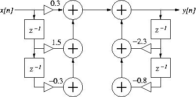
Figure 1: A second-order digital filter.
- Consider the digital filter described by the block diagram in Fig. 1 above:
- Write the difference equation for the filter.
- Use this difference equation to manually calculate the first 7 values of the filter's impulse response (show your calculations).
- In four lines or less (one instruction per line), write Matlab syntax to define the filter and calculate its impulse response (minimum of 50 values).
- Add one more line of Matlab syntax to calculate and plot the filter frequency response (magnitude and phase).
- Derive the transfer function for the filter.
- Find the roots of the transfer function denominator and use those values to discuss the stability of the filter.
- Find the range of values for the a1 coefficient (in a difference equation of the form y[n] = b0 x[n] + b1 x[n-1] + b2 x[n-2] - a1 y[n-1] - a2 y[n-2]) such that the filter is always stable. Keep all the other coefficient values as specified in Fig. 1. Show all steps of the derivation of your answer.
[5 pts]
- Write a Matlab script (not a function) that implements an integer-length delay line in an iterative, single-sample computational context (using a for loop). Define input and output vectors x and y, respectively, and take one sample from x as input to the delayline (which should be implemented as a circular buffer) and write one sample from the delayline to y each iteration. Use one or two pointers to read/write values to/from the delayline during each iteration. Your script needs to work for arbitrary input vector sizes and delay length values. The delay-line length and input vector should be specified at the top of the script. [5 pts]

| © 2004-2024 McGill University. All Rights Reserved.
Maintained by Gary P. Scavone.
|

