Next: Doppler Effect Up: Delay-Based Effects Previous: Delay-Based Effects
![$\displaystyle y[n] = x[n] + g x[n - M[n]],
$](img31.png)
![$M[n]$](img32.png) is the time-varying length of a delay line and
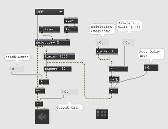
is the time-varying length of a delay line and  is the “depth” of the flanging effect. A flanger block diagram is shown in Fig. 6.
, must change continuously and smoothly through time, it is necessary to make use of an interpolating delay line.
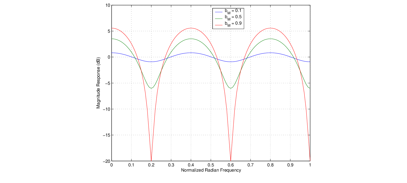
 , there are
  peaks in the frequency response, centered about the frequencies
 . Between these peaks, there are notches at intervals of
  Hz.
Hz.
changes over time, the peaks and notches of the comb response are compressed and expanded. The spectrum of a sound passing through the flanger is thus accentuated and deaccentuated by frequency region in a time-varying manner.
![$\displaystyle M[n] = M_{0} \cdot (1 + A \sin[2 \pi f n T_s]),
$](img40.png)
 is the flanger “rate” in Hz,
  is the “excursion” (maximum delay swing),
  is the average delay-line length that controls the average notch density, and
  is the sample period.
 , the peaks and notches of the comb filter trade places. In practice, is normally contrained to the interval
 ![$[0,1]$](img45.png) and the option of sign inversion is provided by a “phase inversion” switch.
and the option of sign inversion is provided by a “phase inversion” switch.

| ©2004-2024 McGill University. All Rights Reserved. Maintained by Gary P. Scavone. |
![\begin{figure}\begin{center}
\begin{picture}(3.9,0.8)
\put(0.27,0){\epsfig{fil...
...3.0,0.41){$g$}
\put (3.9,0.26){$y[n]$}
\end{picture} \end{center}
\end{figure}](img34.png)