Next: Lossy Wave Propagation Up: Digital Waveguide Theory Previous: Sampled Traveling Waves
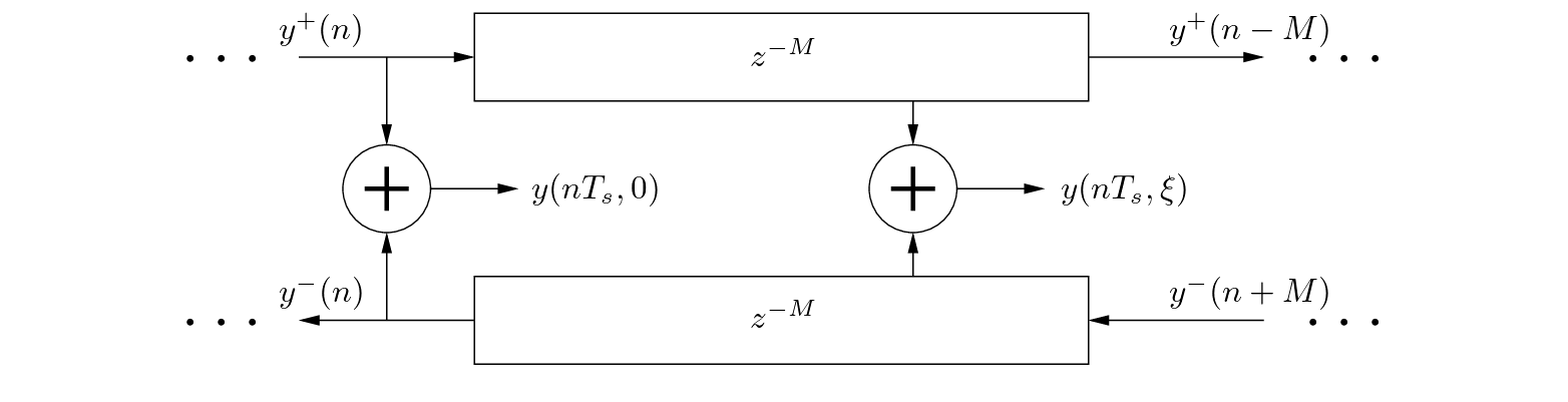
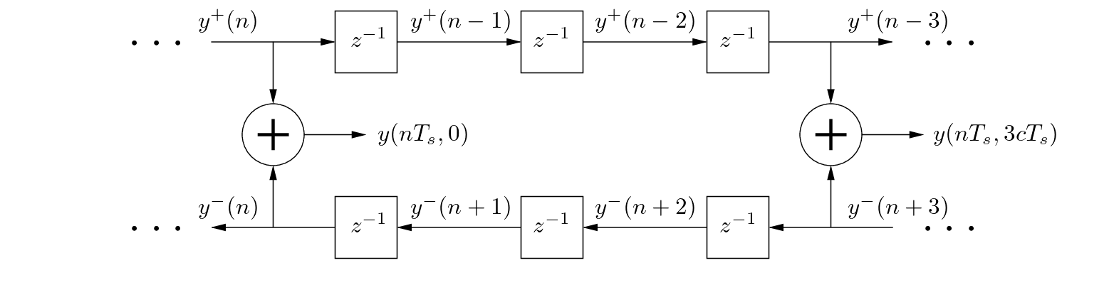
![$y^{+}[(n - m)T_s] = y^{+}(n - m)$](img107.png) can be interpreted as the output of an
can be interpreted as the output of an  -sample delay line of input
  . Similarly, the term
![$y^{-}[(n + m)T_s] = y^{-}(n + m)$](img109.png) can be interpreted as the input to an -sample delay line with output
can be interpreted as the input to an -sample delay line with output  .
.
 |

| ©2004-2024 McGill University. All Rights Reserved. Maintained by Gary P. Scavone. |