Adachi and Sato give steps for the implementation of this model, which are then implemented in the Matlab code, written by Vincent Fréour and edited for use in this project, available here. These steps are summarized below, and comments in the code indicate where each step is implemented. The equations referenced are stated in the previous section, “Model Description.”
Assuming that ξ, p, plip, Uacoust, Ulip, and Slip are known at all times earlier than the present, solve the equation of lip motion (1) defined in the previous section, and find the new ξ, or lip location, for the next timestep. In this implementation, the x- and y-coordinated of ξ are calculated separately.
Calculate the new Slip and Ulip defined by equations (5) and (6) from the previous section.
With the new Slip and Ulip, and past data of p and from U = Uacoust + Ulip, solve the flow equation, given by the sum of (7) and (8), and the feedback equation (10) simultaneously to obtain the new p and Uacoust.
Solve (8) to obtain the new plip.
Update the time by one step, then return to (1).
This implementation does not include the extra conditions imposed upon the lip dynamics when the lips are closed: that the quality factor should change from 3.0 to 0.5, and that an additional restoring force with stiffness 3k should be added along the y-axis.
The parameters used in Adachi and Sato (1996) are summarized in Table 1.
| Symbol | Parameter name | Value |
|---|---|---|
| c | speed of sound | 3x10² m/s |
| ρ | average air density | 1.2 kg/m3 |
| Scup | area of mouthpiece entryway | 2.3x10⁻⁴ m2 |
| b | width of lip opening | 7.0x10⁻³ m |
| d | thickness of lips | 2.0x10⁻³ m |
| ξjoint | lip joint position | (0, 4.0)x10-3 m |
| ξequilx | x coord. of lip rest position | 1.0x10⁻³ m |
| ξequily | y coord. of lip rest position | (-0.1 - 2.0)x10-3 cm |
| Q | lip quality factor | 3.0 on the open-lip condition, 0.5 on the closed-lip condition |
| flip | lip resonance frequency | 60-700 Hz |
| m | lip mass | 1.5/((2π)2flip) kg |
| k | stiffness of lips | 1.5 flip N/m |
| p0 | blowing pressure | 2.0-5.0 kPa |
While Adachi and Sato use a modeled trumpet impedance in both their 1995 and 1996 papers, derived using transfer matrix methods, this implementation uses a measured trumpet impedance.
The impedance measurement used for these calculations is from a Bach Stradivarius B flat trumpet with a modified lead pipe, measured using a CapteurZ measurement system from the Centre de Transfert de Technologie du Mans. The measurement was made using a logarithmic sine sweep from 50 to 4000 Hz, so a sampling rate of 8000 Hz was used for the impedance processing and simulations.
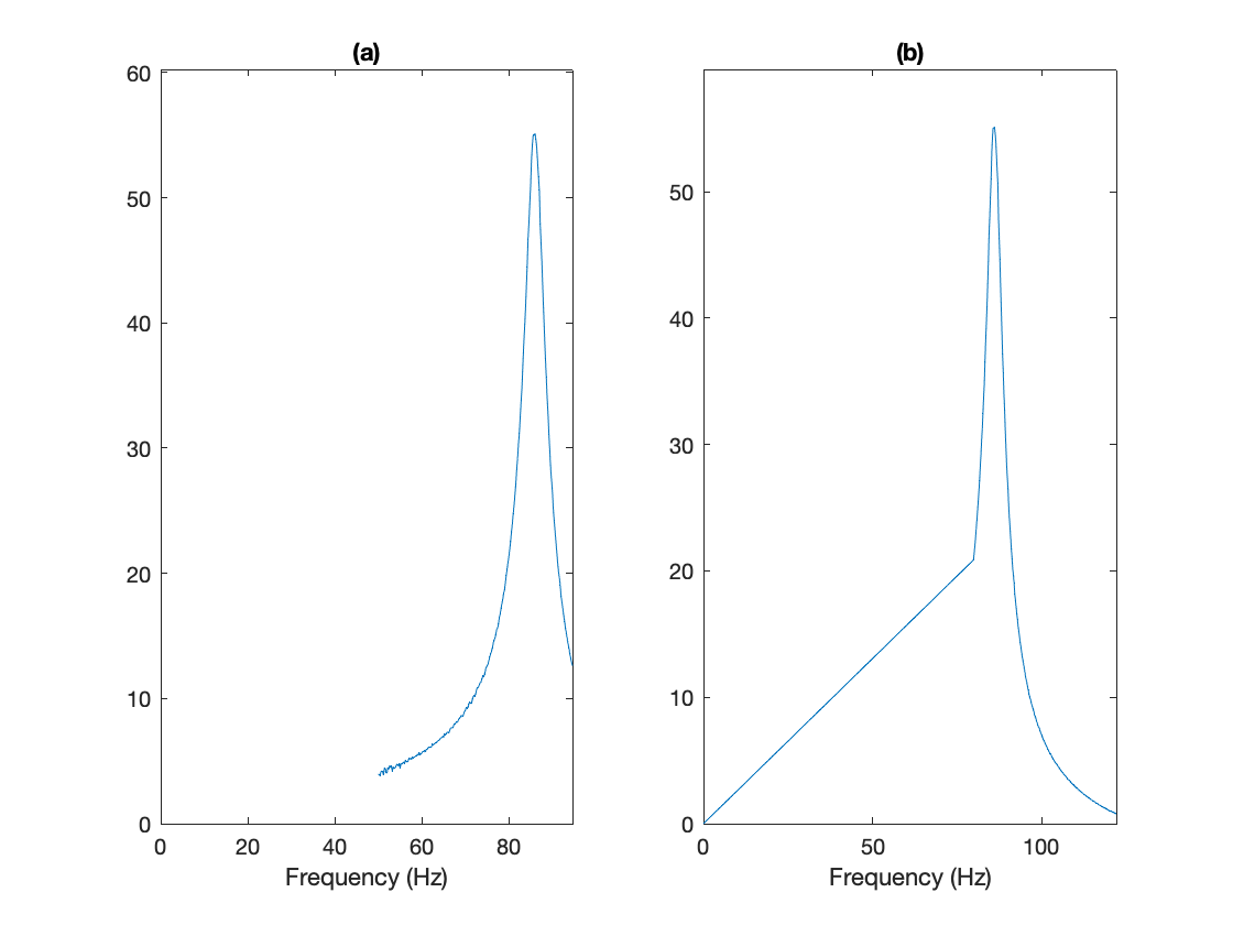
Some minor processing was performed on the measured impedance. First, a length correction of -3mm was added using transfer matrix methods to account for the protrusion of the lips into the mouthpiece. This distance was taken from Fréour’s code without justification for the value chosen, so more investigation would be needed to confirm this value or find a more appropriate choice. The low-frequency section of the impedance measurements, up to 80 Hz, was also interpolated and smoothed linearly, to fill the gap from 0 to 50 Hz before the measured impedance begins and to smooth the lowest 30 Hz of measured frequencies. Figure 2 shows the comparison between the measured and smoothed impedances.