Backward Finite Differences

The Finite Difference technique replaces derivative expressions in differential equations with discrete-time difference approximations.

• The backward finite difference (FD) approximation is given by:
  $$\frac{d}{dt}x(t) \stackrel{\Delta}{=} \lim_{\delta \rightarrow 0} \frac{x(t) - x(t-\delta)}{\delta} \approx \frac{x[n] - x[n-1]}{T_s}$$
  where T is the sampling period.

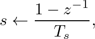
• In the frequency-domain, the FD approximation is defined by the mapping:
  $$s \leftarrow \frac{1 - z^{-1}}{T_s},$$
  where s is the Laplace Transform frequency variable and z is the z-Transform frequency variable.

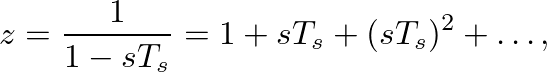
• The inverse finite difference substitution is given by:
  $$z = \frac{1}{1 - s T_s} = 1 + sT_s + (sT_s)^2 + \ldots,$$

• The FD approximation maps analog dc (s=0) to digital dc (z=1).

• By noting that the FD approximation maps an infinite analog frequency ($s=\infty$) to z=0, it should be clear that non-zero poles and zeros are warped in potentially undesireable ways.

• The FD approximation does not alias because the conformal mapping s = 1 - z^-1 is one to one.

• By applying the FD twice, the second derivative is found as:
  $$\frac{d^2}{dt^2}x(t) \approx \frac{x[n] - 2 x[n-1] +x[n-2]}{T_s^2}$$

• The Matlab example, msd_fd.m, demonstrates the use of the finite difference approach to simulate the motion of the mass-spring-damper system.