Next: Finite-Differences vs. the Bilinear Transform Up: Discretization Methods: Previous: Centered Finite Differences
 onto the discrete-time frequency space
 Continuous-time dc (
 ) maps to discrete-time dc (
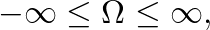
 ) and infinite continuous-time frequency (
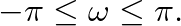
 ) to the Nyquist frequency (
 ). Thus, a nonlinear warping of the frequency axes occurs.
 -axis in the s plane is mapped exactly once around the unit circle of the z plane, no aliasing occurs.
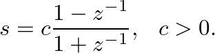
 as
as
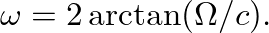
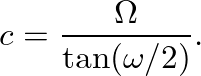
) to the equivalent “digital” frequency ( ), the constant c is found as

| ©2004-2024 McGill University. All Rights Reserved. Maintained by Gary P. Scavone. |