| Homework Submission Process |
- Create a working directory for all your MUMT 307 homework (i.e., mkdir mumt307)
- Create a subdirectory called "homeworkN" (where N = current homework number)
- Put all necessary files, numbered in accordance with the homework questions, in this directory
- When ready to submit, create a "tarball" or "zip" file of the appropriate homework directory (note the addition of a username): tar -czf homeworkN-username.tgz homeworkN/
- Submit the compressed homework directory or files via myCourses
Collaboration Policy: Students can often learn a great deal from their peers. Feel free to seek help from other students (as well as the instructor and TA) when you are having difficulty. But DO NOT COPY assignments. We expect you to write your own patches and code.
Max/MSP Patch Remarks: Design your interfaces in order to group the elements (i.e., buttons, displays, sliders) in an intuitive way. Verify the implementation of the patch so that default parameters are initialized at load time. Add small comments to help the user get started and to understand how the patch works. Test your patch (before delivering it) as if you were a real user that does not know anything about the way it has been implemented. For example, make a copy in another folder, quit Max/MSP, reload the patch and test it. Design each patch in a small window that can be printed on one page only.
Matlab and C++ Code Remarks: Your Matlab and C++ programs should be easy to read and understand. At the top of each script or program, provide the program name, your name, and information about the program and how to use it. For C++ programs, included a g++ compiler statement that can be used to compile the program in the working directory. In your code, be liberal with comments. Even when a program does not execute properly, partial credit may be given based on comments that show good understanding of the issues and ways to approach the solutions. Use the C++ style guide to uniformly format your code.
| Homework #8 | Due: Monday, 25 March 2024 |
- Read pages 277-287 of Computer Music by Dodge & Jerse.
- Choose a sound to model using modal synthesis (one not already in STK). It is best if the object being modeled is excited by striking or plucking and its sound consists of a relatively small number (5-10) of strong resonances (there should be a reasonable sense of pitch to the sound). You will need to obtain a recording of the sound, either from the McGill University Master Samples, the University of Iowa Musical Instrument Samples, Free Sound Samples from wiki.laptop.org, by making a recording yourself, or from another source. Estimate the resonance frequencies, decay rates, and relative gains using the fft functions in Matlab or a spectrum analyzer of your choice. Write a Matlab script that implements a bank of resonant filters to resynthesize the sound (and also show in the script how you performed the parameter estimation). You should also record a "dry" strike sound to use to excite the filters and/or add directly to the resultant sound. Experiment with the parameters to improve the synthesized sound quality. [12 pts]
| Homework #7 | Due: Monday, 18 March 2024 at 22:00 |
- Read pages 90-95, 115-139, 220-258 and 277-287 of Computer Music by Dodge & Jerse.
- Modify the FM brass algorithm demonstrated in stkbrass.cpp to implement the FM Clarinet algorithm ((DUR = 0.5 seconds; fc = 900 Hz; fm = 600 Hz [fc : fm ratio of 3 : 2]; IMIN = 2; IMAX = 4) described on pages 125-127 of Computer Music by Dodge & Jerse (note that IMIN and IMAX refer to minimum and maximum modulation index values). The program should take optional input arguments that specify the fundamental frequency and duration (DUR) of the resulting sound. [10 pts]
| Homework #6 | Due: Monday, 11 March 2024 at 22:00 |
- Create an STK program that generates random pentatonic pitches of short duration. The program can either run in realtime or write the output to a soundfile. Use the SineWave class and an envelope type of your choice (Envelope, Asymp, or ADSR). The program should take command-line arguments to control the duration of each tone and the total duration of the program (see the STK Filters section of the notes for an example program that takes input arguments). Make sure your program provides a usage statement if the necessary arguments are missing or inappropriate values are specified. [5 pts]
| Homework #5 | Due: Monday, 12 February 2024 at 22:00 |
- Read pages 99-100 and 158-167 of Computer Music by Dodge & Jerse.
- In Matlab, create a unit impulse signal and use it as input to a Schroeder allpass filter with g = 0.7 and a delay of 357 samples (given by a difference equation of y[n] = -g x[n] + x[n-M] + g y[n-M]). Then use the output of that filter as input to a feedback comb filter specified by the difference equation y[n] = x[n] - 0.95 y[n-1037]. Plot the resulting impulse response and the corresponding magnitude frequency response. [3 pts]
- Choose a continuously excited sound (ex., wind or bowed-string instruments) to model using additive synthesis. You will need to obtain a recording of the sound (options include the McGill University Master Samples, the University of Iowa Musical Instrument Samples, Free Sound Samples from wiki.laptop.org, by making a recording yourself, or from another source). Single tones are fine. Estimate the time-varying resonance frequencies and amplitudes using the fft or spectrogram functions in Matlab or another software spectrum analyzer. Then resynthesize the sound in either Matlab or Max/MSP using sinusoidal oscillators and the estimated parameters. Include the original soundfile with your submission, as well as the analysis information you derived from it. You should interpolate the sinusoidal amplitudes and frequencies over time as needed. [10 pts]
Note that piece-wise linear envelopes can be generated in Matlab using the interp1 function as follows:
fs = 44100;                      % sample rate
T = 1/fs;                        % sample period
x = [0 30 700 1000];             % time breakpoints in milliseconds
y = [0.0 1.0 0.8 0.0];           % corresponding amplitude breakpoints at times given by vector x
n = 0:44099;                     % time in samples (1 second at 44.1 kHz)
env = interp1(x, y, 1000*n*T);   % scale the time steps to milliseconds
| Homework #4 | Due: Monday, 5 February 2024 at 22:00 |
- Read pages 72-90 and 262-275 of Computer Music by Dodge & Jerse.
- Build a Max/MSP patch that implements a dynamic range compressor as shown in the flow chart below. The compressor should be for monophonic sounds. The patch should process input from either a sinusoidal oscillator or an adc~ object.
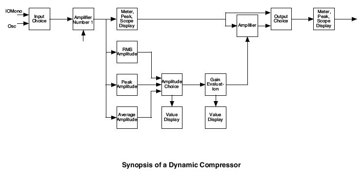
The output signal of the compressor should be a scaled version of the input signal. The scaling is determined by a transfer function relating output signal power (in dB) to input signal power (in dB), parameterized by a threshold T and a compression ratio R, where R = input signal power (in dB) / output signal power (in dB) above the threshold T. When the input signal power is less than the threshold T, R = 1.0 (no compression occurs). Input signals are expected to be amplitude normalized within the range -1.0 to +1.0 so that R = 1.0 for all input signals if T = 0 dB.
The user should be able to:
- Select the input (oscillator - OSC in the diagram - or direct audio input).
- Change the amplitude and the frequency of the oscillator.
- Change the input signal gain.
- Select one of three ways to evaluate the signal amplitude (peak, average, rms).
- Modify the "transfer function" of the gain compression via sliders for R and T.
- Turn the compressor function on/off.
The gain evaluation, or compression curve, should be displayed using the Max function object. The display of the "transfer function" will be the output level in dB on the y-axis and the input level in dB on the x-axis. The ranges will be defined from -100 to 0 dB for both axes. Since the minimum value for the x-axis when using the function object is 0, you should implement a shift-in, shift-out offset before and after the function object. The compression curve display should be automatically updated when modifications are made to the compression ratio and threshold slider values. [20 pts]
| Homework #3 | Due: Monday, 29 January 2024 at 22:00 |
- Read pages 289-308 of Computer Music by Dodge & Jerse.
- Build a Max/MSP patch that simulates a very simple monophonic synthesizer. This synthesizer must include a controlled generator and a controlled amplifier.
The user should be able to select any one of the following three waveforms for the generator: sinusoid, sawtooth, or resonant filtered noise. Pitch will be controlled using the Max keyboard (kslider) object and will include a vibrato effect with a frequency modulation rate of 5 to 10 Hz and a frequency deviation of 5-10% (with respect to the fundamental pitch frequency).
A note should continue as long as a key on the kslider is depressed (change the "Display Mode" to "Touchscreen" in the inspector) and then stop when the key is released. Use line~ objects to envelope each note attack and release, with key velocity controlling the attack and release durations (the highest possible velocity will result in the minimum envelope duration, the lowest possible velocity will result in the maximum envelope duration). The interface should include two number boxes to allow the specification of the maximum and minimum attack and release durations (attack and release durations will be the same). Note that a velocity of zero should not produce a sound. Also, the pitch value should control the center frequency of the resonant filtered noise.
Other required features:
- A global output gain to control the overall amplitude.
- A graphical display of the output time-domain signal.
- Sliders to control the vibrato rate and deviation (within the limits mentioned above).
Remarks: Think of the implementation in a modular way (you might use subpatches); design the interface in order to group the parameters into a control front panel (you may use routing objects to clarify the structure of the patch); verify the implementation of the patch so that default parameters are initialized at load time; add small comments to help the user get started and to understand how the patch works; Test your patch (before delivering it) as if you were a real user that does not know anything about the way it has been implemented. For example, make a copy in another folder, quit Max/MSP, reload the patch and test it. Design each patch/subpatch in a small window that can be printed on one page only. [10 pts]
- Write a Matlab script that defines the following two filter structures, as well as plots their frequency responses [2 pts]:
- a. A feedback comb filter given by the difference equation: y[n] = 0.8 x[n] - y[n - 4999].
- b. A second-order allpass filter given by the difference equation: y[n] = 0.81 x[n] - 1.73 x[n-1] + x[n-2] + 1.73 y[n-1] - 0.81 y[n-2].
| Homework #2 | Due: Tuesday, 23 January 2024 at 22:00 |
- Read pages 169-219 of Computer Music by Dodge & Jerse.
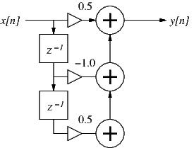
Figure 1: A second-order digital filter.
- Consider the digital filter described by the block diagram in Fig. 1 above:
- Write the difference equation for the filter.
- Using the input signal x[n] = {..., 1, 1, 1, 1, ...}, what is the steady-state gain of the filter at zero frequency?
- Using the input signal x[n] = {..., 1, -1, 1, -1, ...}, what is the steady-state gain of the filter at half the sample rate?
- Is this a FIR or an IIR filter? What general type of filter is it (lowpass, highpass, resonance, shelf, ...)?
- Use the difference equation to calculate the first 5 values of the filter's impulse response (write out the operations by hand).
[2 pts]
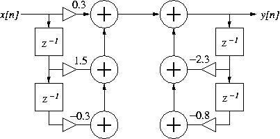
Figure 2: A second-order digital filter.
- Consider the digital filter described by the block diagram in Fig. 2 above:
- Write the difference equation for the filter.
- Use this difference equation to calculate the first 5 values of the filter's impulse response (write out the operations by hand).
- Is the filter stable? Explain your answer.
- In four lines or less (one instruction per line), write Matlab syntax to define the filter and calculate its impulse response (minimum of 50 values).
- Add one more line of Matlab syntax to calculate and plot the filter frequency response (magnitude and phase).
[4 pts]
- Digital Resonance Filters:
- Write Matlab syntax to define a digital resonance filter with a center frequency of 2000 Hz at a sample rate of 44100 Hz (let r = 0.99). The filter gain at the center frequency should be normalized. Verify the design by plotting the filter frequency response.
- Use the Matlab rand function to generate a one-second noise sequence (scale it to a range from -1.0 < x < +1.0 with zero mean) and use this as input to the filter. Use the spectrogram() function to view the spectrum of the resulting filtered noise.
[3 pts]
| Homework #1 | Due: Tuesday, 16 January 2024 at 22:00 |
- Review chapters 1-3 of Computer Music by Dodge & Jerse, pp. 1-71.
- Write a matlab script that performs the following operations on the audio file triangle.wav:
- Use the audioread() function to read the audio file data (signal and sample rate) into Matlab variables.
- Play the audio signal using the soundsc() function (which normalizes the signal level and removes any DC offset).
- Plot the magnitude frequency response of the entire signal on a decibel scale. Provide a title and both x- and y-axis labels.
- Plot the spectrogram of the signal, which displays the frequency content of the signal over time. In order to accomplish this, you can use the Matlab function spectrogram(y, WINDOW, NOVERLAP, NFFT, Fs), where WINDOW = 1024, NOVERLAP=512, NFFT=1024, and Fs is the sample rate of the file. Provide a title on the spectrogram.
[5 pts]
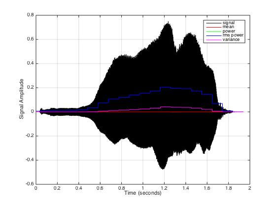
- Write another Matlab script that computes and displays the mean, power, rms power, and variance of the waveform in trumpet.wav. These metrics should be calculated over "blocks" of M samples (define M near the top of your script with a default value of 4275) and the plotted metric values should be superposed over the signal as horizontal lines that vary every M samples. Provide a legend in the plot. The Matlab reshape() function can be used to simplify the calculations. The example sinemetrics.m script should provide a good starting point. In the end, the plot should look like the figure below. [7 pts]

| ©2004-2024 McGill University. All Rights Reserved.
Maintained by Gary P. Scavone.
|