Next: Simulation Results Up: Bowed String Modeling Previous: The Bowing Mechanism
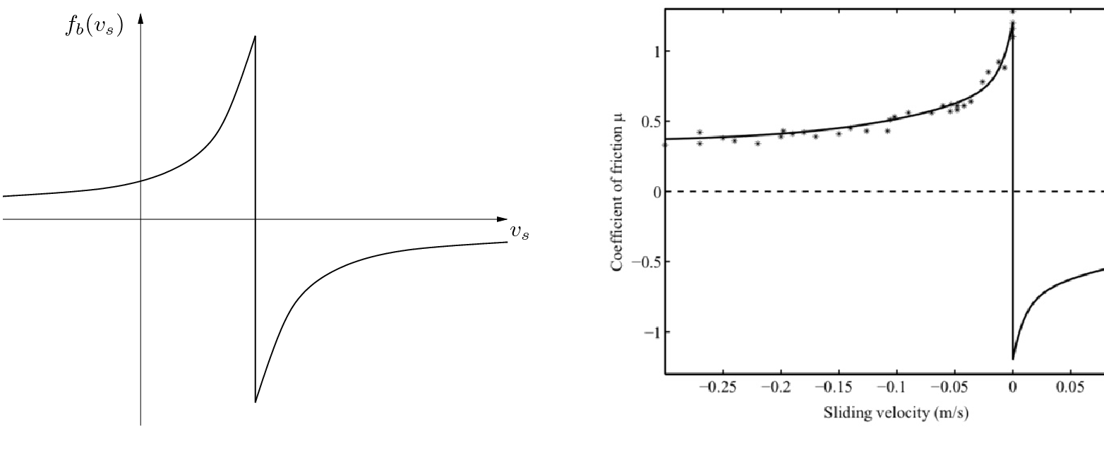 |
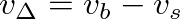 , the difference between the bow and string velocities.
 (the point of infinite slope in the figure). In this case, the friction force is based primarily on static friction.
 , the string is “slipping” and the friction force is based roughly on kinetic friction, which is significantly less than the static friction (especially when rosin is applied to the bow).
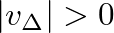
![$f_{s} = R_s [v_{s}^{+} - v_{s}^{-}] = R_s [v_{s} - 2v_{s}^{-}]$](img6.png) , where
, where  is the string wave impedance.
|

| ©2004-2024 McGill University. All Rights Reserved. Maintained by Gary P. Scavone. |