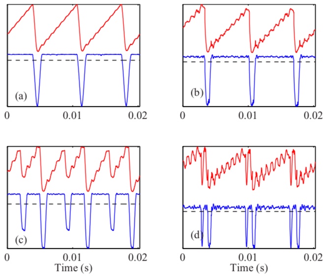
Figure 6:
Simulated waveforms for a cello open D string: (a),(b) Helmholtz motion with two values of normal force; (c) Double slip motion; (d) Double flyback motion. Upper trace: bridge force (shifted vertically for clarity); lower trace: string velocity at bowed point; dashed line: zero line for velocity trace (from Woodhouse (2014)).
Figure 6 provides a few examples of simulated string force (at bridge) and velocity (at bow) waveforms. The model allows some torsional motion of the string, so the velocity of the string's centre-line need not be exactly constant during sticking: the string can roll on the sticking bow.
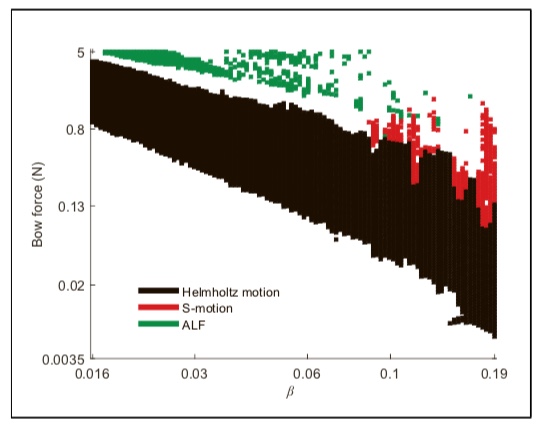
An example of a simulated Schelleng diagram is shown in Fig. 7 (from Mansour et al. (2016a)). S-motion is similar to the Helmholtz motion in that there is a single stick and slip per nominal period, but the s-motion involves large ripples superposed on the expected sawtooth bridge force (it occurs when the bow position is close to a string nodal point). An ALF note is a musical tone with a frequency much lower than that of the first string mode and requires very precise control of the bow parameters to achieve. Decaying, double-slip and raucous regimes are omitted for clarity.
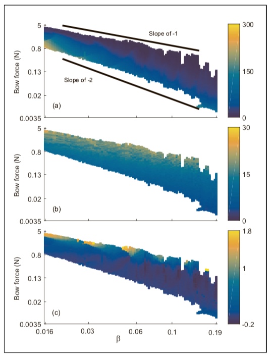
Other aspects of the playing behaviour can be deduced from such simulations. Figure 8 presents (a) The increase in the slip-to-stick ratio as a percentage of its theoretical value (unit x100 s/s), (b) the spectral centroid relative to the fundamental frequency (unit Hz/Hz), and (c) the pitch flattening as a percentage of the fundamental frequency (unit 100 Hz/Hz). The theoretical slopes for the minimum and maximum bow force are shown in (a) by thick diagonal lines to guide the eye (from Mansour et al. (2016a)).
Mansour et al. (2016a) then goes on to compare the variation of these metrics with various modular model additions or subtractions, such as finger-stopping, longitudinal string vibrations, bow-stick flexibility, dual-polarisation, no torsion, no stiffness, rigid terminations, and thermal friction model.