Next: The Body Model Up: Bowed String Modeling Previous: Simulation Results
 must at all times balance with the reactive force of the string (
![$f_s = R_s [v_s^+ - v_s^-]$](img10.png) ).
).
 .
.
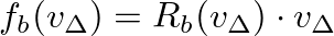
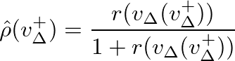
 ) to allow an expression of the form:
![$\displaystyle R_b(v_{\Delta}) \cdot v_{\Delta} = R_s \left[ v_{\Delta}^{+} - v_{\Delta} \right]
$](img13.png)
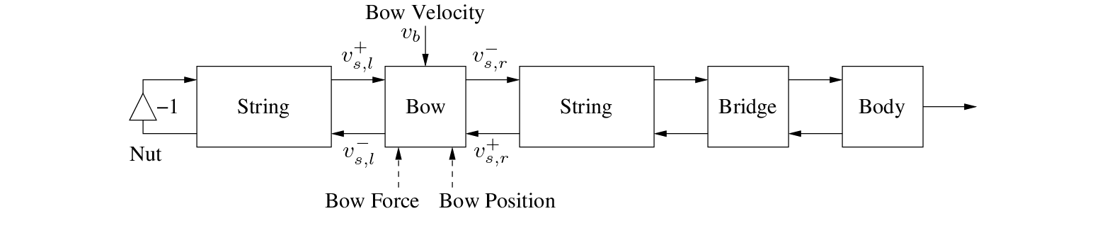
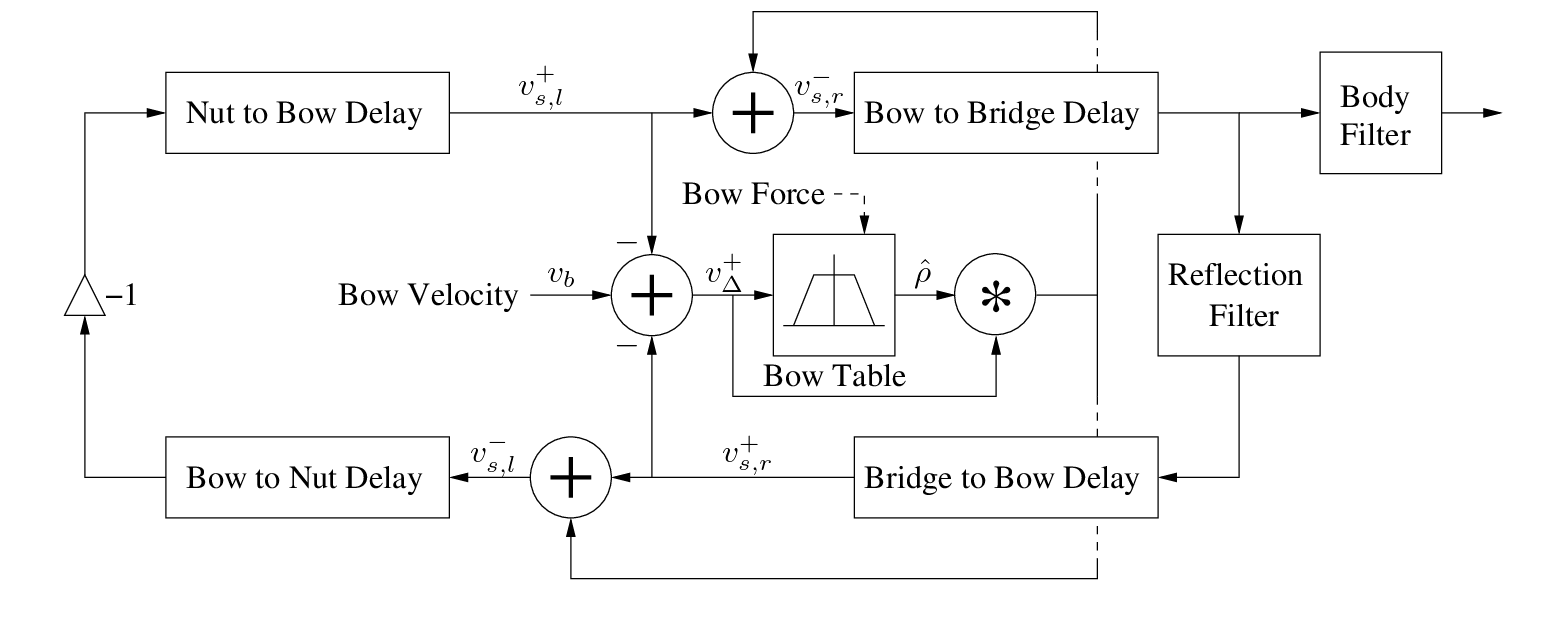
![$v_{\Delta}^{+} = v_b - [v_{s,l}^{+} + v_{s,r}^+]$](img14.png) .
.
 superscripts.
 .
.
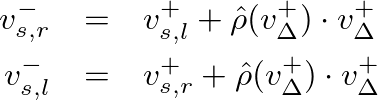
 and
and  are computed so that the physical string velocity is equal to
  .
.

| ©2004-2024 McGill University. All Rights Reserved. Maintained by Gary P. Scavone. |