Next: Wave Reflections and “Echo” Up: Sound and Wave Phenomena Previous: Reflection, Diffraction, Refraction and Doppler
 between source and listener will result in a time delay of
  seconds (where
  is the speed of sound propagation).
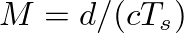 , where
  is the digital sample period (and
  is the sampling rate in samples per second).
 represents the distance traveled by sound in a single sample period, which is about 7 millimeters at a sample rate of 48000 Hz.
 (due to spherical spreading), where is the distance of the wavefront from its source. Thus, when simulating the pressure of spherical wavefronts, an additional “spreading” factor should be added as shown in Fig. 3.

| ©2004-2024 McGill University. All Rights Reserved. Maintained by Gary P. Scavone. |

![\begin{figure}\begin{center}
\begin{picture}(3.9,0.5)
\put(0.26,0){\epsfig{fil...
...0.13){$g^{M}$}
\put (3.9,0.13){$y[n]$}
\end{picture} \end{center}
\end{figure}](img20.png)
![\begin{figure}\begin{center}
\begin{picture}(3.9,0.5)
\put(0.26,0){\epsfig{fil...
...2,0.29){$1/d$}
\put (3.9,0.13){$y[n]$}
\end{picture} \end{center}
\end{figure}](img21.png)