The previous discussion was based on the use of digital delay lines with integer sample delay lengths. In many contexts, it is necessary to compute the output of a delay line at fractional delay-line lengths.
While signal values in a delay line are stored at integer multiples of the sample period , it is possible to apply interpolation techniques to approximate values between those in memory.
The most common interpolation techniques used in conjunction with delay lines are linear interpolation and allpass interpolation.
Linear interpolation is an efficient technique for determining sample values at fractional delay line lengths. Intermediate values between two neighboring samples are found by “drawing” a line that connects those two samples and returning values along that line.
Let be a number between 0 and 1 that indicates how far to interpolate a signal between time and time . The linearly interpolated value
is given by:
A block diagram for linear interpolation is shown in Fig. 14.
Figure 14:
A linearly interpolated delay line.
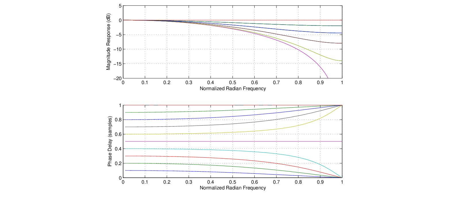
The magnitude and phase delay for a linear interpolation filter, calculated with the Matlab script interpolate.m, is shown in Fig. 15 for fractional delays between 0 and 1.
Figure 15:
Magnitude and phase delay for linear interpolation with fractional delays between 0 and 1.
From the frequency response plots, it is apparent that linear interpolation becomes less accurate for high frequencies. In particular, the “artificial” attenuation that is introduced at higher frequencies can be problematic in feedback loops where the loop gain should be close to 1.
Linear interpolation is also known as first-order Lagrange interpolation. Lagrange interpolators are FIR filter structures. Higher order Lagrange interpolators can be more accurate but are less efficient to implement.