Next: Refinements Up: Reed Valve Modeling Previous: The Reed as a Mass-Spring-Damper
 is the reed channel width,
  is the time-varying reed position, calculated from Eq. (29), and
  is the equilibrium tip opening.
 is the traveling-wave pressure entering the reed junction from the downstream air column.
 is the computational sample rate.
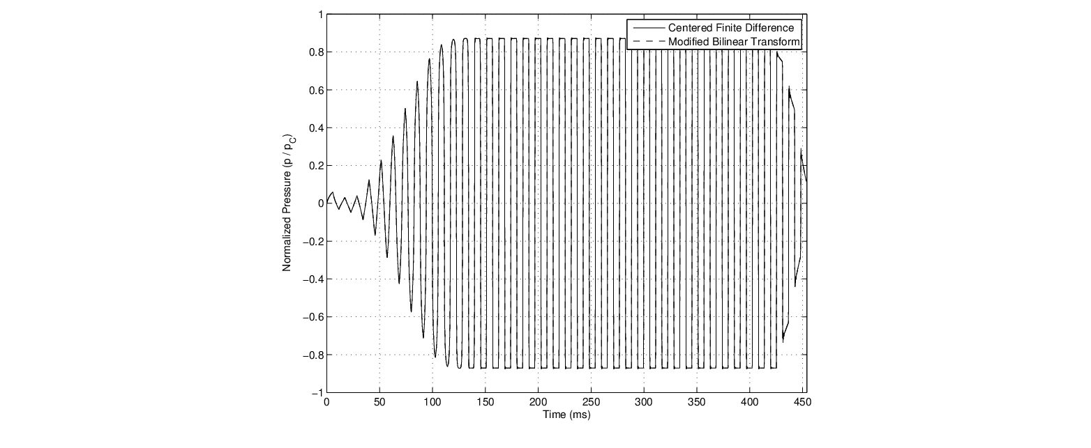
 , limiting its use at low sample rates and/or with high reed resonance frequencies.
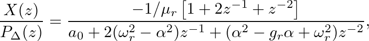
 and
and  is the bilinear transform constant that controls frequency warping.
 .
.
 (or at frequencies of 0 and
  Hz). While this result is often desirable for digital resonators, we can modify the numerator terms without affecting the essential behavior and stability of the resonator.
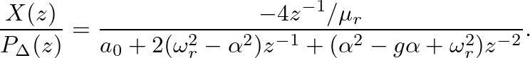
 Hz and
  Hz.
Hz.
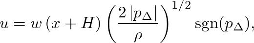
 |
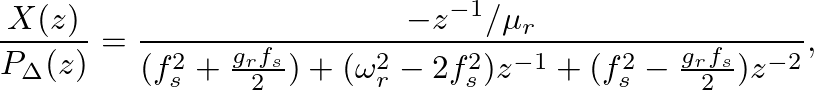
 , it is possible to explicitly solve Eqs. (32) and (21), as noted in Guillemain et al. (2005), by an expression of the form
 (36)
(36)
 and
and
 can be determined at the beginning of each iteration from constant and past known values.
 ,
,  is set to zero and
 .
.
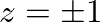
Hz and Hz.

| ©2004-2024 McGill University. All Rights Reserved. Maintained by Gary P. Scavone. |
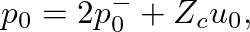
![\begin{figure}\begin{center}
\begin{picture}(4.0,1.0)
\put(0.21,0){\epsfig{file...
...){$\delta[n]$}
\put(0.42,0.94){$Z_{c}$}
\end{picture} \end{center}
\end{figure}](img131.png)